
Estimating Calendar Year Correlation in Loss Triangles
reserving
correlation
Empirical analysis of the calendar year correlation structure in loss reserving triangles using the CAS Loss Reserve Database.
Loss reserving models often assume independence between cells in a loss triangle. In practice, common factors like inflation, legal changes, and economic conditions create correlations between cells, particularly those falling within the same calendar year diagonal. This post quantifies that correlation structure using 200 paid loss triangles from the CAS Loss Reserve Database.
The Block Autoregressive Correlation Structure
A natural correlation structure for loss triangles is the “block autoregressive” model, where:
- Cells on the same calendar year diagonal have correlation \(\rho\)
- Cells separated by \(k\) calendar years have correlation \(\rho^{k+1}\)
This structure captures the intuition that calendar year effects (inflation, judicial trends, economic conditions) create dependencies between cells processed in the same period, with correlation decaying geometrically as calendar years diverge.
The correlation matrix for a small triangle illustrates this structure:
Data: The Meyers 200 Triangles
We use the 200 paid loss triangles from Glenn Meyers’ testing subset of the CAS Loss Reserve Database, accessed via the reservetestr package. These triangles span four major lines of business:
- Commercial Auto (50 triangles)
- Personal Auto (50 triangles)
- Workers Compensation (50 triangles)
- Other Liability (50 triangles)
Each triangle contains accident years 1988-1997 with development periods from 12 to 120 months, giving 55 observable cells per triangle.
| Line of Business | Triangles | Accident Years | Development Periods | |
|---|---|---|---|---|
| 0 | Commercial Auto | 50 | 1988-1997 | 12-120 months |
| 1 | Personal Auto | 50 | 1988-1997 | 12-120 months |
| 2 | Workers Compensation | 50 | 1988-1997 | 12-120 months |
| 3 | Other Liability | 50 | 1988-1997 | 12-120 months |
Methodology
To estimate the calendar year correlation structure, we:
- Extract incremental paid losses from each triangle and apply a log transformation
- Compute residuals by removing accident year and development period effects using a log-linear model: \(\log(\text{incremental}) \sim \text{AY} + \text{dev}\)
- Calculate Spearman rank correlations between all pairs of cells across the 200 triangles
- Group correlations by calendar year distance between cell pairs
- Estimate confidence intervals via bootstrap resampling of triangles
Using residuals removes the systematic effects of accident year (loss trend) and development period (payment pattern), isolating the calendar year effect. Spearman correlation is robust to outliers and non-normality in the loss data.
Results
Overall Correlation Structure
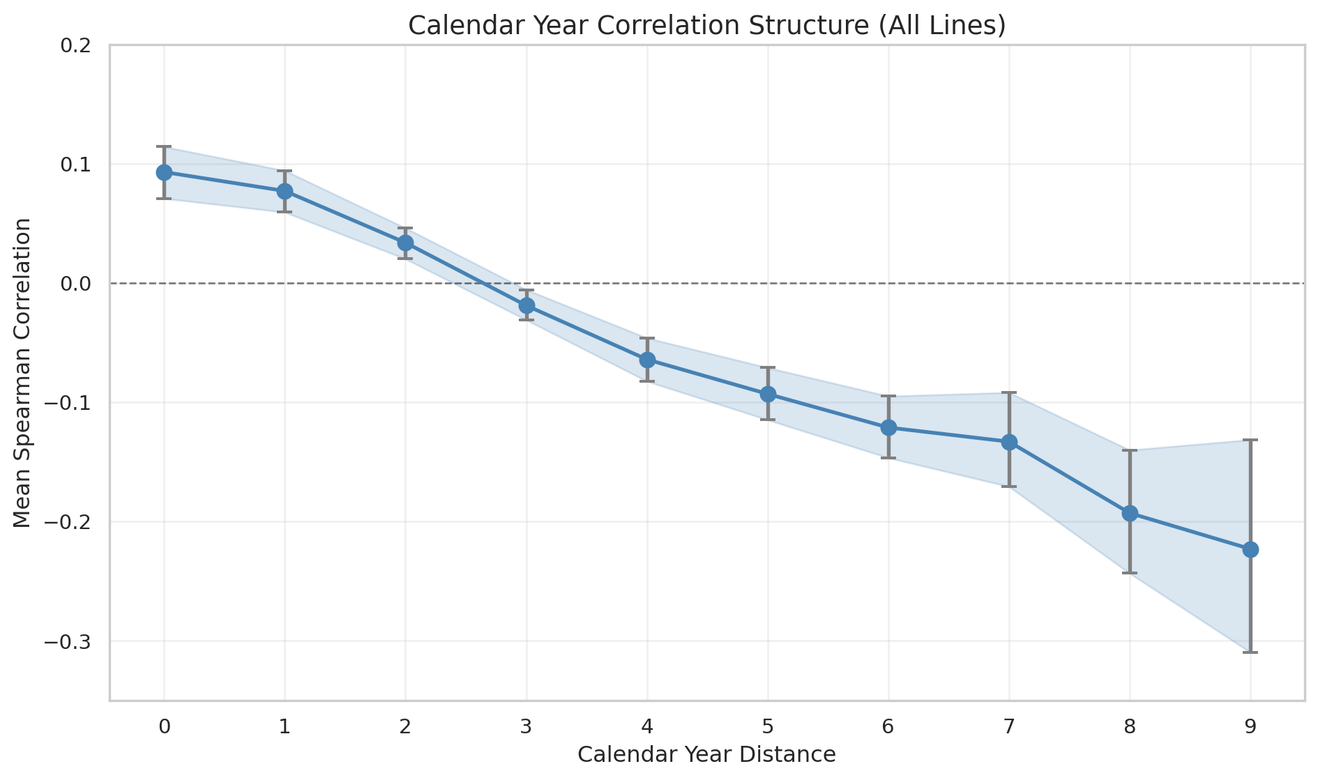
The following table shows the mean Spearman correlation between cell pairs, grouped by the calendar year distance between them. Distance 0 represents cells on the same calendar year diagonal; distance 1 represents adjacent calendar years, and so on.
| CY Distance | Mean Correlation | 95% CI | SE | Cell Pairs | |
|---|---|---|---|---|---|
| 0 | 0 | 0.093 | [0.071, 0.114] | 0.0108 | 126 |
| 1 | 1 | 0.077 | [0.059, 0.094] | 0.0087 | 273 |
| 2 | 2 | 0.034 | [0.020, 0.046] | 0.0067 | 238 |
| 3 | 3 | -0.019 | [-0.031, -0.006] | 0.0065 | 191 |
| 4 | 4 | -0.064 | [-0.082, -0.046] | 0.0093 | 147 |
| 5 | 5 | -0.093 | [-0.115, -0.071] | 0.0111 | 107 |
| 6 | 6 | -0.121 | [-0.147, -0.095] | 0.0133 | 72 |
| 7 | 7 | -0.133 | [-0.171, -0.092] | 0.0202 | 43 |
| 8 | 8 | -0.193 | [-0.243, -0.140] | 0.0258 | 21 |
| 9 | 9 | -0.223 | [-0.310, -0.131] | 0.0454 | 7 |
The key finding is that cells on the same calendar year diagonal have a positive correlation of approximately 0.09 (95% CI: 0.07 to 0.11). This correlation:
- Remains positive for adjacent calendar years (distance 1-2)
- Crosses zero around distance 3
- Becomes increasingly negative for more distant calendar years
Correlation by Line of Business
The calendar year correlation varies substantially across lines of business:
| Line of Business | ρ (Same CY) | 95% CI | ρ (Adjacent CY) | Triangles | |
|---|---|---|---|---|---|
| 0 | Commercial Auto | 0.118 | [0.075, 0.157] | 0.096 | 50 |
| 1 | Personal Auto | 0.175 | [0.132, 0.216] | 0.173 | 50 |
| 2 | Workers Compensation | 0.053 | [0.015, 0.094] | 0.026 | 50 |
| 3 | Other Liability | 0.072 | [0.034, 0.116] | 0.031 | 50 |
| 4 | All Lines | 0.093 | [0.071, 0.114] | 0.077 | 200 |
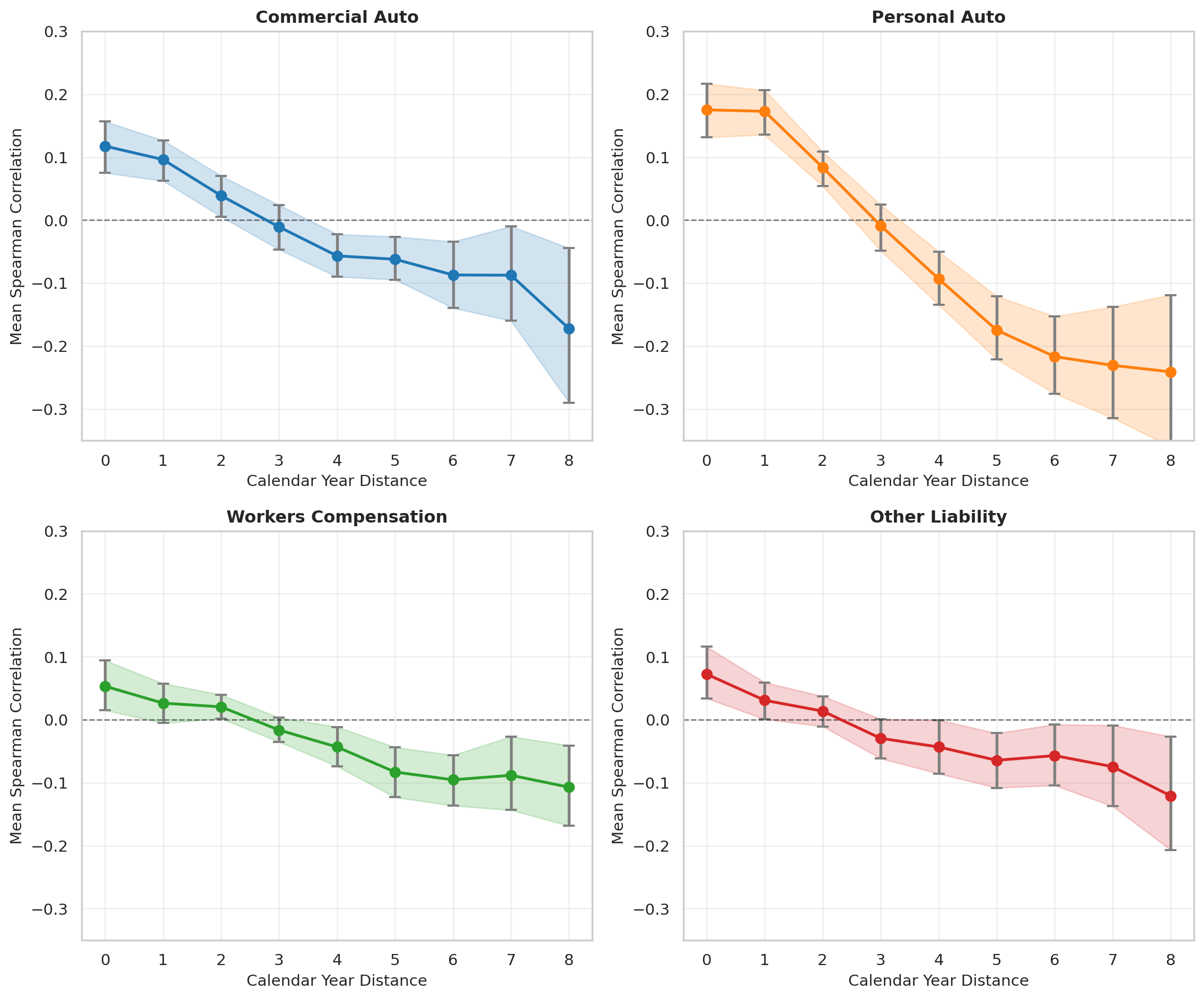
The variation across lines likely reflects differences in:
- Claim duration: Personal Auto claims settle quickly, making calendar year effects more concentrated
- Economic sensitivity: Auto lines may be more responsive to economic cycles
- Regulatory environment: Workers Compensation is heavily regulated, potentially dampening calendar year variation
Comparison to Block AR Model
The simple block autoregressive model predicts that correlation should decay as \(\rho^{k+1}\) for cells \(k\) calendar years apart. Let’s compare the empirical pattern to this theoretical structure:
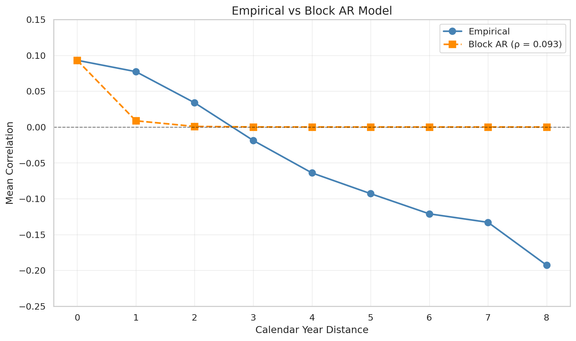
The comparison reveals that:
- The block AR model captures the general decay pattern but predicts faster decay than observed
- Correlation at distance 1 is higher than predicted, suggesting adjacent calendar years are more similar than the simple model assumes
- The sign reversal at larger distances is not captured by the block AR model, which predicts positive (though small) correlations at all distances
This suggests that a more flexible correlation structure may be needed to fully capture the empirical pattern, perhaps incorporating mean-reversion effects that create negative correlations between distant calendar years.
Implications for Reserve Estimation
These findings have practical implications for stochastic loss reserving:
Ignoring calendar year correlation understates reserve uncertainty. The positive correlation between cells on the same diagonal means that unfavorable calendar year effects (higher inflation, adverse legal developments) will simultaneously affect multiple cells, creating correlated reserve errors.
The magnitude of correlation varies by line. Personal Auto reserves may require stronger correlation assumptions (\(\rho \approx 0.17\)) than Workers Compensation (\(\rho \approx 0.05\)).
Simple block AR structures may oversimplify. The empirical evidence suggests correlation decays more slowly than \(\rho^{k+1}\) for nearby calendar years, and the sign reversal at larger distances indicates mean-reversion effects not captured by the simple model.
Reasonable parameter ranges for simulation. When simulating correlated loss triangles, a same-diagonal correlation of \(\rho \in [0.05, 0.20]\) appears reasonable based on this analysis, with the specific value depending on line of business.
Technical Notes
Standardization: We use residuals from a simple log-linear model rather than raw values to remove systematic accident year and development period effects that would otherwise dominate the correlation structure.
Spearman correlation: We use rank correlation to be robust to outliers and non-normality in the loss distributions. Pearson correlations yield similar but slightly noisier results.
Bootstrap inference: Confidence intervals are computed by resampling triangles (not cells) to preserve the within-triangle correlation structure.
Negative correlations at large distances: This pattern suggests mean-reversion in calendar year effects—a year with unusually high losses tends to be followed (eventually) by years with lower losses. This could reflect mean-reverting inflation or correction of reserve estimates.
The code for this analysis uses the reservetestr package for data access and standard Python libraries (pandas, scipy, matplotlib) for analysis and visualization.