Correlation Assumptions in Economic Capital Models
capital
economic-capital
correlation
solvency
A data-driven analysis of correlation assumptions across risk types in P&C insurance capital models, drawing from Solvency II, AM Best BCAR, and S&P methodologies.
Building an economic capital model requires making assumptions about how risks interact. The correlation between underwriting risk, reserve risk, credit risk, equity risk, and interest rate risk fundamentally determines the diversification benefit—and thus the required capital—for an insurance company. Yet these correlation assumptions are often treated as black boxes inherited from regulatory frameworks.
This post examines the correlation matrices used by major rating agencies and regulators, explores their empirical foundations (or lack thereof), and demonstrates the sensitivity of capital requirements to these assumptions.
The Correlation Problem
When aggregating standalone capital charges for different risk types, the aggregation formula is critical. The most common approach uses a variance-covariance structure:
\[ \text{Total Capital} = \sqrt{\sum_{i,j} \rho_{ij} \cdot C_i \cdot C_j} \]
where \(C_i\) is the capital charge for risk \(i\) and \(\rho_{ij}\) is the correlation between risks \(i\) and \(j\).
At the extremes:
- Perfect correlation (\(\rho = 1\)): Capital adds linearly: \(C_{\text{total}} = \sum_i C_i\)
- Perfect independence (\(\rho = 0\)): Capital adds in quadrature: \(C_{\text{total}} = \sqrt{\sum_i C_i^2}\)
For a typical P&C insurer, the difference between these assumptions can represent 30-50% of required capital.
Solvency II Standard Formula Correlations
The Solvency II Standard Formula provides the most transparent correlation framework, with matrices codified in the Delegated Regulation (EU) 2015/35.
Basic SCR Correlation Matrix
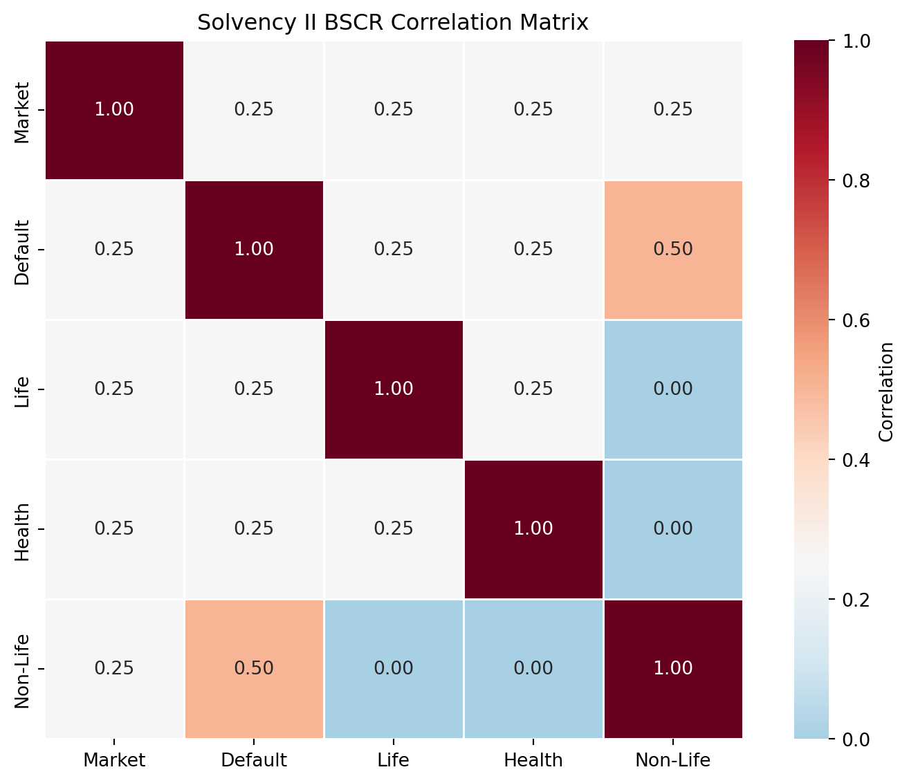
The Basic Solvency Capital Requirement (BSCR) aggregates five major risk modules using this correlation matrix:
Key observations from the BSCR matrix:
- Life and Non-Life have zero correlation: The regulation assumes life insurance and P&C underwriting risks are independent, reflecting their different exposure drivers
- Default and Non-Life have 0.5 correlation: Higher than other pairings, capturing the relationship between reinsurance/policyholder credit risk and the underwriting cycle
- Market risk correlates uniformly (0.25): With all other modules, a simplified assumption
Market Risk Sub-Module Correlations
Within the Market risk module, Solvency II provides a more nuanced correlation structure that depends on the interest rate scenario:
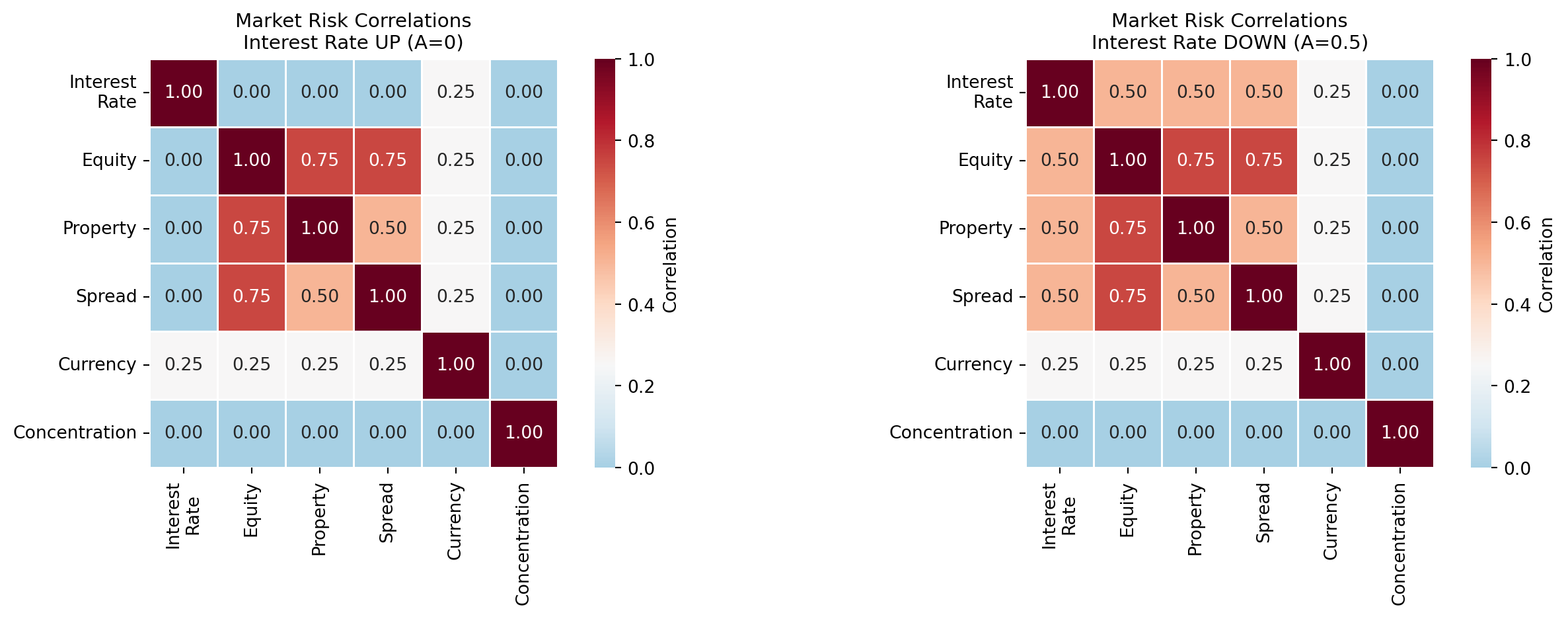
The scenario-dependent correlation is one of Solvency II’s more sophisticated features. In falling rate environments, equities and credit spreads tend to move together with rates (all falling in risk-off scenarios), justifying the 0.5 correlation. In rising rate environments, equity and spread behavior is more idiosyncratic relative to rates.
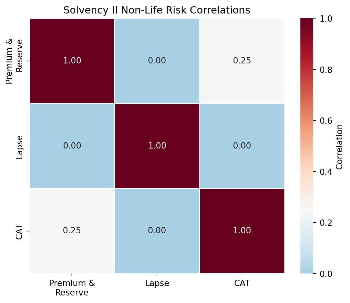
Non-Life Underwriting Risk Correlations
For P&C insurers, the Non-Life underwriting risk module aggregates:
- Premium and Reserve Risk: Combined as a single sub-module
- Catastrophe Risk: Natural catastrophe, man-made, and other catastrophe risks
AM Best BCAR Approach
AM Best’s Best’s Capital Adequacy Ratio (BCAR) model uses a different approach, applying a covariance adjustment through a “square root rule” with explicit correlation between certain components:
Net Required Capital Formula: \[ \text{NRC} = \sqrt{B_1^2 + B_2^2 + B_3^2 + (0.5 \cdot B_4)^2 + [(0.5 \cdot B_4) + B_5]^2 + B_6^2 + B_8^2} + B_7 \]
Where: - \(B_1\): Fixed income securities risk - \(B_2\): Equity securities risk - \(B_3\): Interest rate risk - \(B_4\): Credit risk (split and correlated with reserve risk) - \(B_5\): Reserve risk - \(B_6\): Premium risk - \(B_7\): Business risk (excluded from covariance) - \(B_8\): Catastrophe risk
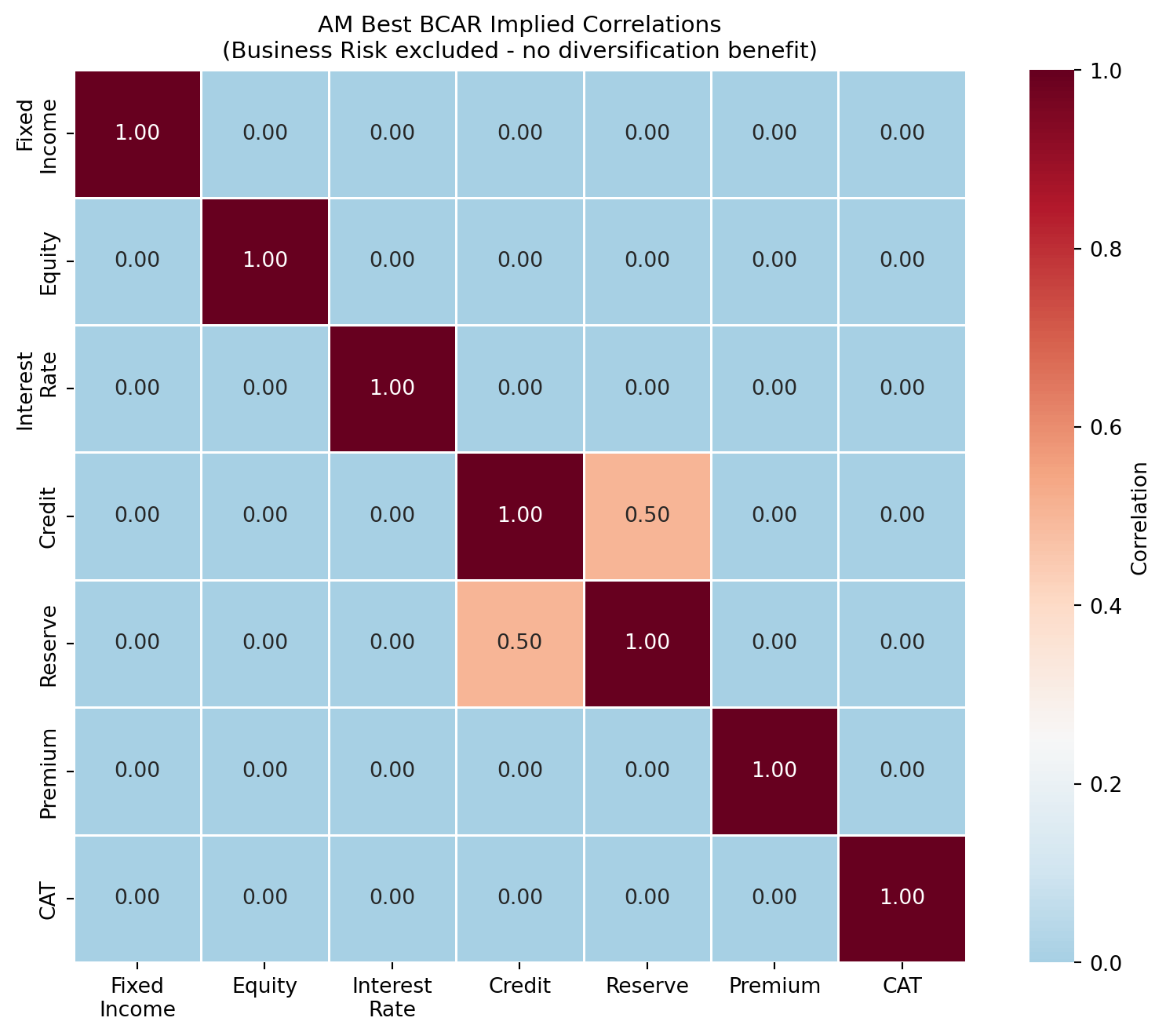
Key features of the AM Best approach:
- Most risk components are independent: The square root formula treats most risks as uncorrelated
- Credit and Reserve risk are linked: The formula structure implies these move together
- Business risk receives no diversification: Added after the square root calculation
- VaR calibration at multiple levels: 95%, 99%, 99.5%, and 99.6% confidence levels
S&P Global Capital Model
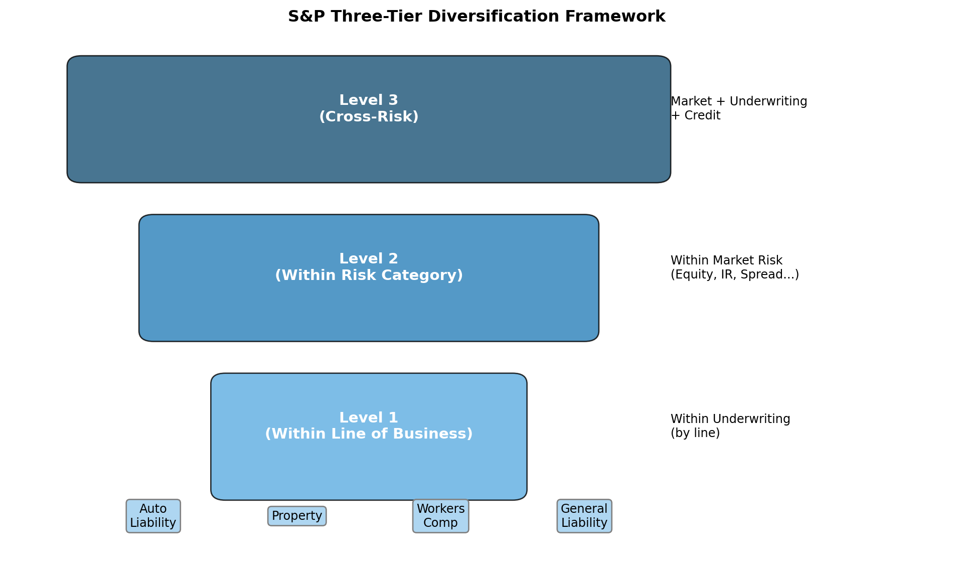
S&P’s 2023 updated criteria introduced a three-tier diversification framework:
- Level 1: Diversification within lines of business
- Level 2: Diversification within risk categories (market risk, underwriting risk, etc.)
- Level 3: Diversification between major risk categories
S&P’s key correlation features:
- Higher confidence levels: 99.5% (moderate), 99.8% (substantial), 99.95% (severe), 99.99% (extreme)
- Updated correlation factors: Increased diversification benefits within life technical and market risks
- New Level 3 diversification: Explicit correlation matrix between major risk categories
Comparative Analysis
How do these frameworks compare for a typical P&C insurer? Let’s construct a representative risk profile and examine capital under different correlation assumptions:
| Risk Category | Capital Charge (%) | Description | |
|---|---|---|---|
| 0 | Underwriting (Premium) | 15% | Risk from current year premiums |
| 1 | Underwriting (Reserve) | 25% | Risk from reserve development |
| 2 | Credit/Default | 10% | Counterparty and reinsurance credit |
| 3 | Equity Risk | 12% | Stock market volatility |
| 4 | Interest Rate Risk | 8% | Duration mismatch |
| 5 | Spread Risk | 10% | Credit spread widening |
| 6 | Property Risk | 5% | Real estate holdings |
| 7 | Catastrophe Risk | 15% | Natural and man-made catastrophes |
Impact of Correlation Uncertainty
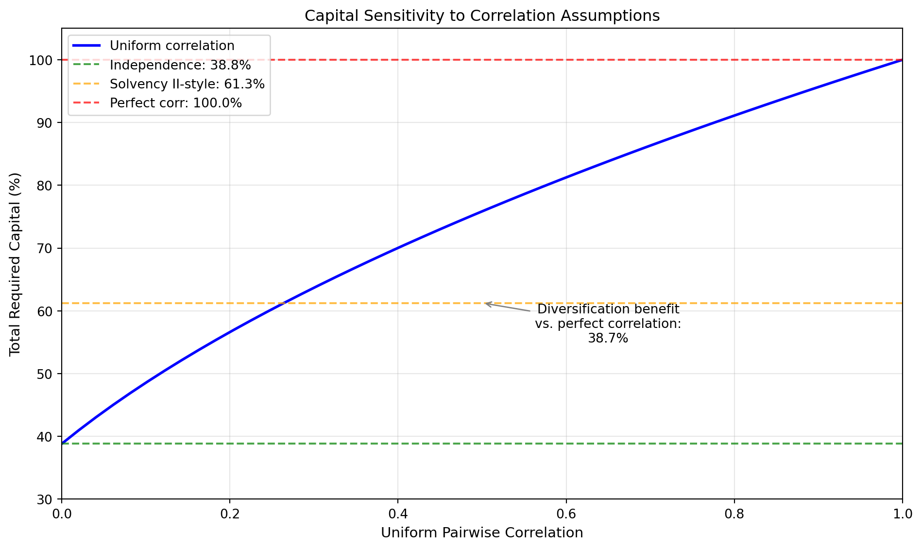
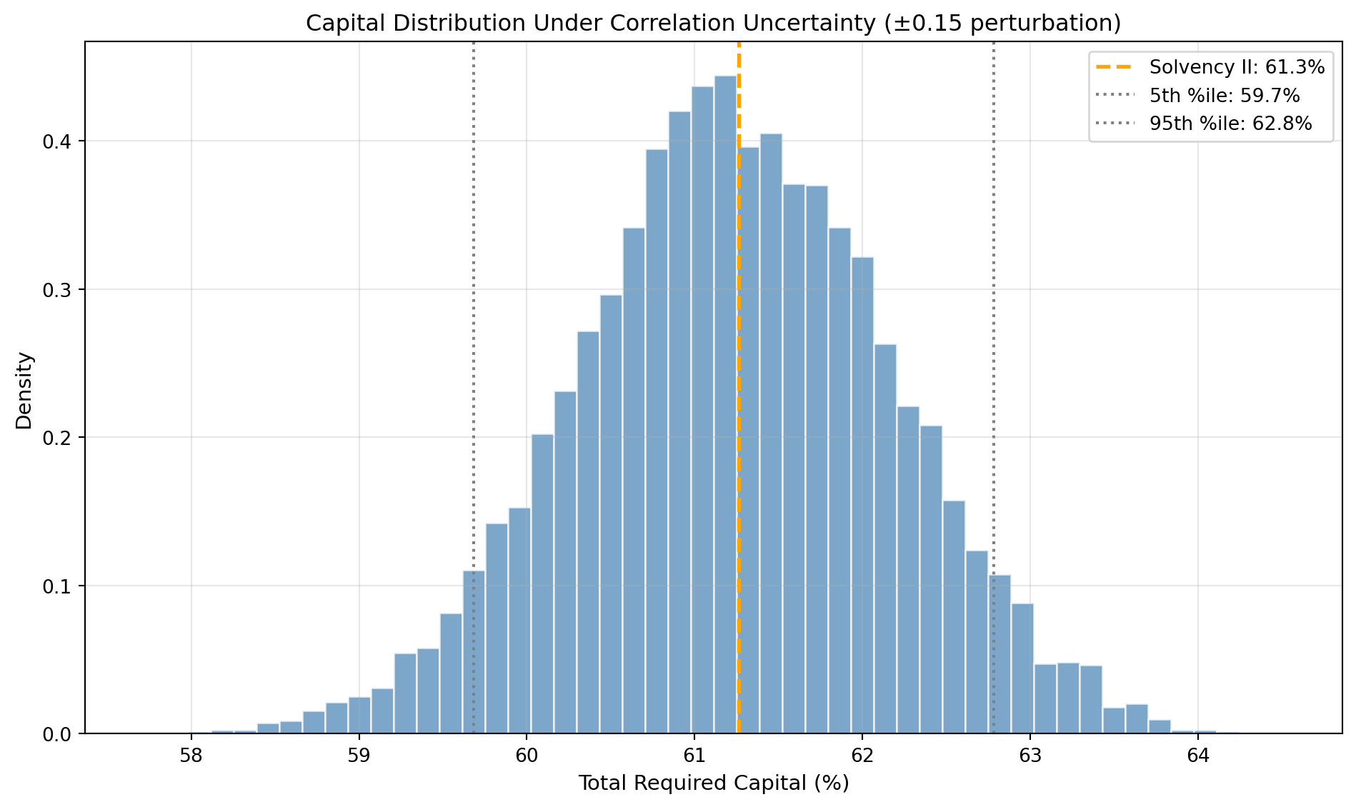
The correlation assumptions have significant capital implications, but their empirical foundation is often weak. Let’s examine how uncertainty in correlation parameters propagates to capital uncertainty:
| Scenario | Capital (%) | Diversification Benefit | |
|---|---|---|---|
| 0 | Independence | 38.8 | 61.2% |
| 1 | Solvency II | 61.3 | 38.7% |
| 2 | Perfect Correlation | 100.0 | 0% |
| 3 | Correlation Uncertainty (5th-95th) | 59.7 - 62.8 | 38.8% (mean) |
Which Correlations Matter Most?
Not all pairwise correlations have equal impact on total capital. Let’s identify the most influential correlation parameters:
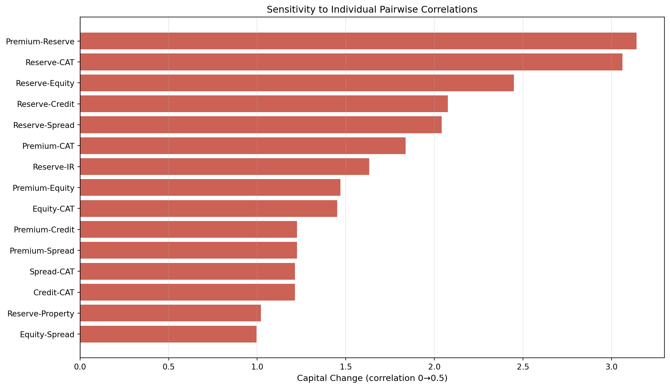
The analysis reveals that Reserve-Premium and Reserve-Credit correlations have the most significant capital impact, reflecting that reserve risk is often the largest standalone charge.
Empirical Evidence on Correlations
The regulatory correlations are often criticized for weak empirical foundations. What does actual data suggest?
Underwriting-Investment Correlation
Academic research on the relationship between underwriting and investment risks shows mixed results:
- Underwriting and investment risks in the property-liability insurance industry found no significant relationship between underwriting and investment risks in pre-9/11 data
- Canadian P&C insurance research shows equity investment and reinsurance underwriting have opposite effects on capital levels
This suggests the 0.25 correlation between Market and Non-Life risk in Solvency II may be conservative.
Interest Rate and Equity Correlation
The scenario-dependent correlation in Solvency II (0 in up-rate, 0.5 in down-rate scenarios) has stronger empirical support. During financial crises:
- Interest rates fall (flight to quality)
- Equity markets decline
- Credit spreads widen
These effects create positive correlation in tail scenarios, justifying higher correlations at the 99.5% VaR level.
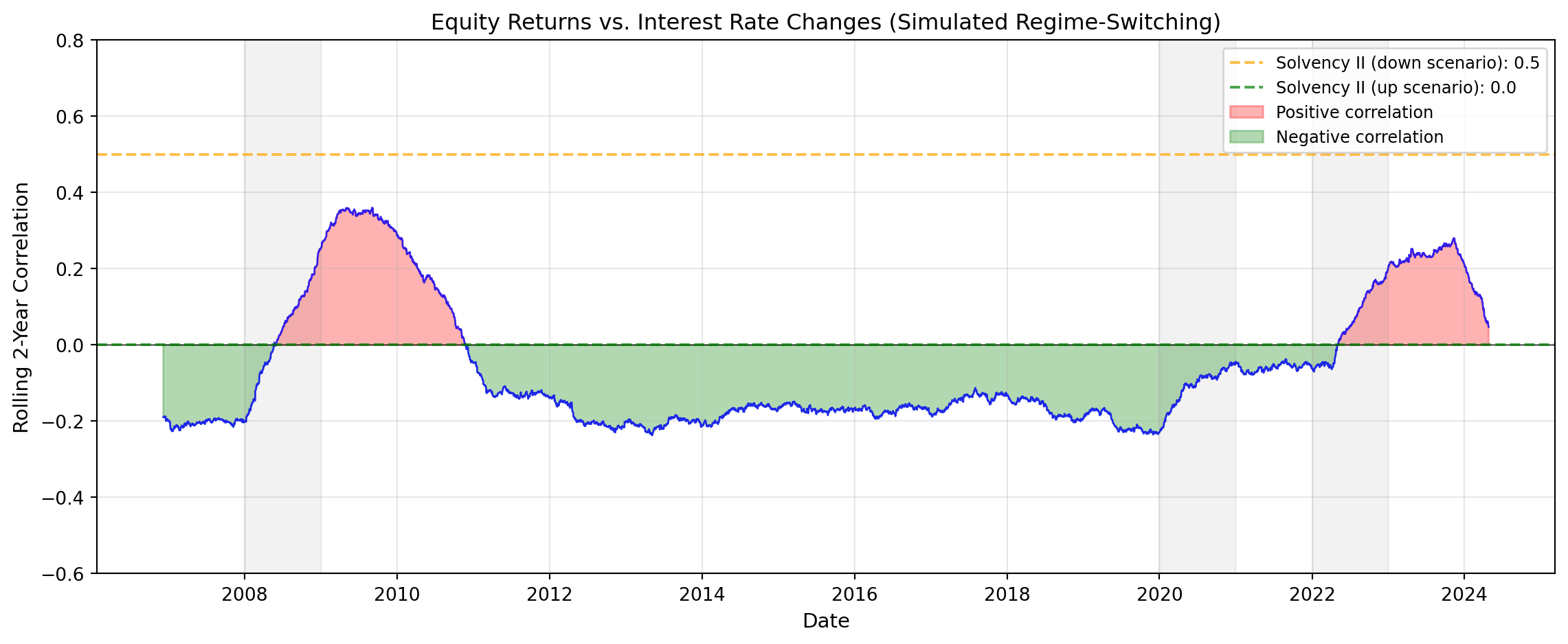
This simulation captures the key empirical observation: equity-rate correlations are regime-dependent. In normal markets, there’s often a negative correlation (rates up = equities up, reflecting economic growth). During crises, the correlation turns positive (rates down + equities down, reflecting flight-to-quality and risk-off dynamics). This justifies Solvency II’s scenario-dependent approach.
Practical Recommendations
Based on this analysis, here are recommendations for parameterizing correlations in your economic capital model:
1. Start with Regulatory Frameworks
Use Solvency II correlations as a baseline—they represent regulatory consensus and facilitate comparison with public disclosures:
| Risk Pair | Solvency II | Recommended Range |
|---|---|---|
| Market - Non-Life | 0.25 | 0.15 - 0.35 |
| Credit - Non-Life | 0.50 | 0.40 - 0.60 |
| Premium - Reserve | 0.50 | 0.40 - 0.70 |
| Equity - Spread | 0.75 | 0.60 - 0.85 |
| CAT - Other | 0.00 - 0.25 | 0.00 - 0.30 |
2. Use Scenario-Dependent Correlations
Following Solvency II’s approach for market risk, consider stress-dependent correlations:
- Normal conditions: Use lower correlations reflecting day-to-day behavior
- Stress conditions: Use higher correlations reflecting crisis dynamics
3. Conduct Sensitivity Analysis
Given the capital impact, always report results under multiple correlation scenarios:
- Independence (best case)
- Base case (regulatory or internal estimate)
- Stressed correlations (worst case)
4. Focus Validation Efforts
Prioritize empirical validation for the correlations with highest capital sensitivity:
- Reserve - Premium
- Reserve - Credit
- Equity - Spread
Summary
| Framework | VaR Level | Correlation Approach | Key Features | Transparency | |
|---|---|---|---|---|---|
| 0 | Solvency II | 99.5% | Explicit matrices at module and sub-module levels | Scenario-dependent IR correlations; 0.25/0.50 ... | High (published in regulation) |
| 1 | AM Best BCAR | 95% - 99.6% | Implicit through covariance formula structure | Square root aggregation; some risks excluded f... | Medium (formula-implied) |
| 2 | S&P | 99.5% - 99.99% | Three-tier diversification framework | Updated 2023 criteria with enhanced diversific... | Medium (criteria document) |
Correlation assumptions are among the most consequential—and least empirically grounded—parameters in economic capital models. For a typical P&C insurer, the choice between independence and perfect correlation can swing capital requirements by 40-50%. Even modest uncertainty in correlation parameters (±0.15) creates a 10+ percentage point range in required capital.
The prudent approach is to use regulatory frameworks as a starting point, understand which correlations have the largest impact on your specific portfolio, and maintain explicit documentation of assumptions and their sensitivities.