Bayesian Chain Ladder

Use Bayesian methods to replicate the Chain Ladder reserving method

Published

January 12, 2019

Goal

The goal of this post is to use the rstanarm package to run a Bayesian Chain Ladder reserving method on the CAS Loss Reserve Database. The cross classified generalized linear model (GLM) formulation of the Chain Ladder will be used.

See STOCHASTIC LOSS RESERVING USING GENERALIZED LINEAR MODELS for a description of the cross classified GLM formulation. The same example triangle used in the monograph is also used in this post.

In future posts, we will investigate the results further and explore extensions to the baseline model.

Data


# devtools::install_github("problemofpoints/reservetestr")
library(tidyverse)
library(ChainLadder)
library(reservetestr)
library(broom)
library(broom.mixed)
library(rstanarm)
library(bayesplot)
library(popformatting)
library(patchwork)

# set ggplot2 theme
popformatting::gg_set_theme()

# pull in the subset of the CAS loss reserve database used by Meyers
cas_triangle_db_meyers <- reservetestr::cas_loss_reserve_db %>%
  reservetestr::get_meyers_subset()

# extract sample paid loss triangle to use
sample_company <-  cas_triangle_db_meyers %>%
  dplyr::filter(group_id == 7080 & line == "wkcomp")

paid_triangle <- sample_company %>%
  pull(train_tri_set) %>% 
  .[[1]] %>% 
  .$paid

paid_triangle_no_exposure <- paid_triangle
attr(paid_triangle_no_exposure, "exposure") <- NULL

paid_triangle
#>       dev_lag
#> acc_yr     1      2      3      4      5      6      7      8      9     10
#>   1988 41821  76550  96697 112662 123947 129871 134646 138388 141823 144781
#>   1989 48167  87662 112106 130284 141124 148503 154186 158944 162903     NA
#>   1990 52058  99517 126876 144792 156240 165086 170955 176346     NA     NA
#>   1991 57251 106761 133797 154668 168972 179524 187266     NA     NA     NA
#>   1992 59213 113342 142908 165392 179506 189506     NA     NA     NA     NA
#>   1993 59475 111551 138387 160719 175475     NA     NA     NA     NA     NA
#>   1994 65607 110255 137317 159972     NA     NA     NA     NA     NA     NA
#>   1995 56748  96063 122811     NA     NA     NA     NA     NA     NA     NA
#>   1996 52212  92242     NA     NA     NA     NA     NA     NA     NA     NA
#>   1997 43962     NA     NA     NA     NA     NA     NA     NA     NA     NA
#> attr(,"exposure")
#>  [1] 195712 212194 219796 249595 268293 316726 344287 356880 313412 261261

Standard chain ladder estimate

We can use the glmReserve function from the ChainLadder package to produce the standard Chain Ladder reserve estimate. This method provides both a point estimate and a distribution of estimates, using a bootstrapping approach. This function uses the cross classified over-dispersed Poisson GLM formulation applied to an incremental paid loss triangle, which exactly re-produces the traditional Chain Ladder reserve estimate. For convenience in producing the Bayesian equivalent, we use the Negative Binomial distribution instead of the over-dispersed Poisson. This is done by setting the nb parameter to TRUE in glmReserve. We still achieve mean results essentially equivalent to the traditional chain ladder estimate.

est_chainladder_nb <- glmReserve(paid_triangle_no_exposure, 
                                 var.power = 1, link.power = 0, cum = TRUE, 
                                 mse.method = "bootstrap", nsim = 5000,
                                 nb = TRUE)

est_chainladder_nb$summary %>%
  rownames_to_column("Acc Yr") %>% 
  mutate_at(c(2,4:6), popformatting::number_format) %>% 
  flextable::regulartable() %>% 
  popformatting::ft_theme(add_w = 0.0, add_h = 0.00, add_h_header = 0.00) %>%
  flextable::bg(i = nrow(est_chainladder_nb$summary), 
                bg = "#F2F2F2", part = "body") %>% 
  popformatting::add_title_header("Chain ladder reserve estimate", 
                                  font_size = 18) %>% 
  flextable::fontsize(size = 16, part = "all")

Chain ladder reserve estimate
Acc Yr	Latest	Dev.To.Date	Ultimate	IBNR	S.E	CV
1989	162,903	0.9794376	166,323	3,420	333	0.09749463
1990	176,346	0.9559292	184,476	8,130	542	0.06664080
1991	187,266	0.9255245	202,335	15,069	823	0.05462254
1992	189,506	0.8931800	212,170	22,664	1,126	0.04966852
1993	175,475	0.8464949	207,296	31,821	1,480	0.04651688
1994	159,972	0.7788088	205,406	45,434	2,164	0.04763981
1995	122,811	0.6710177	183,022	60,211	3,047	0.05060250
1996	92,242	0.5329782	173,069	80,827	4,705	0.05820747
1997	43,962	0.2934360	149,818	105,856	8,211	0.07756789
total	1,310,483	0.7782358	1,683,915	373,432	11,626	0.03113416

The total Chain Ladder reserve estimate for this triangle is 373,432 with an overall coefficient of variation (CV) of 3.11%.

We can also output the underlying GLM formula and fitted parameters.

summary(est_chainladder_nb, type = "model")
#> 
#> Call:
#> glm.nb(formula = value ~ factor(origin) + factor(dev), data = ldaFit, 
#>     init.theta = 331.5546543, link = log)
#> 
#> Deviance Residuals: 
#>     Min       1Q   Median       3Q      Max  
#> -2.0547  -0.8338   0.0000   0.7548   2.4347  
#> 
#> Coefficients:
#>                    Estimate Std. Error z value Pr(>|z|)    
#> (Intercept)        10.64796    0.02678 397.680  < 2e-16 ***
#> factor(origin)1989  0.14524    0.02639   5.503 3.73e-08 ***
#> factor(origin)1990  0.24120    0.02752   8.765  < 2e-16 ***
#> factor(origin)1991  0.36897    0.02875  12.832  < 2e-16 ***
#> factor(origin)1992  0.39068    0.03025  12.913  < 2e-16 ***
#> factor(origin)1993  0.36907    0.03218  11.471  < 2e-16 ***
#> factor(origin)1994  0.35424    0.03480  10.180  < 2e-16 ***
#> factor(origin)1995  0.24495    0.03873   6.325 2.53e-10 ***
#> factor(origin)1996  0.18578    0.04547   4.086 4.39e-05 ***
#> factor(origin)1997  0.04312    0.06128   0.704    0.482    
#> factor(dev)2       -0.20610    0.02598  -7.934 2.13e-15 ***
#> factor(dev)3       -0.74477    0.02721 -27.376  < 2e-16 ***
#> factor(dev)4       -1.01574    0.02854 -35.591  < 2e-16 ***
#> factor(dev)5       -1.44957    0.03017 -48.041  < 2e-16 ***
#> factor(dev)6       -1.84320    0.03228 -57.094  < 2e-16 ***
#> factor(dev)7       -2.14799    0.03517 -61.072  < 2e-16 ***
#> factor(dev)8       -2.34589    0.03944 -59.476  < 2e-16 ***
#> factor(dev)9       -2.50783    0.04676 -53.636  < 2e-16 ***
#> factor(dev)10      -2.65570    0.06380 -41.622  < 2e-16 ***
#> ---
#> Signif. codes:  0 '***' 0.001 '**' 0.01 '*' 0.05 '.' 0.1 ' ' 1
#> 
#> (Dispersion parameter for Negative Binomial(331.5547) family taken to be 1)
#> 
#>     Null deviance: 11754.138  on 54  degrees of freedom
#> Residual deviance:    54.947  on 36  degrees of freedom
#> AIC: 962.24
#> 
#> Number of Fisher Scoring iterations: 1
#> 
#> 
#>               Theta:  331.6 
#>           Std. Err.:  64.7 
#> 
#>  2 x log-likelihood:  -922.243

The factor(origin) parameters, often also known as alpha parameters, represent the accident year level of loss. The factor(dev) parameters (or beta parameters) represent the development year direction. We can re-arrange the fitted development year parameters to re-create the standard chain ladder link ratios, as shown in the table below.

model_params <- broom::tidy(est_chainladder_nb$model) %>%
  separate(term, into = c("factor","variable","value"), "\\(|\\)") %>%
  mutate(value = as.numeric(value)) %>%
  mutate(value = case_when(variable == "Intercept" ~ 1,
                          variable == "origin" ~  value - 1988 + 1, 
                          variable == "dev" ~ value)) %>%
  mutate(variable = case_when(variable == "Intercept" ~ "origin",
                              TRUE ~ variable)) %>%
  select(variable, value, estimate) %>%
  bind_rows(tibble(variable = "dev",value=1,estimate=0)) %>% 
  mutate(estimate2 = case_when(variable == "origin" & value == 1 ~ estimate[1],
                               variable == "origin" & value != 1 ~ estimate[1]+estimate,
                               variable == "dev" ~ estimate)) %>%
  mutate(estimate3 = case_when(variable == "origin" ~ exp(estimate2),
                               variable == "dev" ~ exp(estimate))) %>% 
  mutate(estimate_normalized = case_when(variable == "origin" ~ 
                                           exp(estimate2) * sum(.$estimate3[.$variable=="dev"]),
                               variable == "dev" ~ 
                                 estimate3 / sum(.$estimate3[.$variable=="dev"]))) %>% 
  arrange(variable, value)

model_params_link <- model_params %>%
  filter(variable == "dev") %>% 
  mutate(link = lead(cumsum(estimate3) / lag(cumsum(estimate3)))) 

model_params_link %>% 
  select(`Dev period` = value, `LN(Betas)` = estimate, Betas = estimate3, 
         Normalized = estimate_normalized, `Link ratios` = link) %>% 
  mutate_at(2:5, number_format, digits = 3) %>% 
  flextable::regulartable() %>% 
  ft_theme() %>% 
  add_title_header("GLM parameters - development factors", font_size = 18) %>% 
  flextable::fontsize(size = 16, part = "all")

GLM parameters - development factors
Dev period	LN(Betas)	Betas	Normalized	Link ratios
1	0.000	1.000	0.293	1.814
2	-0.206	0.814	0.239	1.262
3	-0.745	0.475	0.139	1.158
4	-1.016	0.362	0.106	1.089
5	-1.450	0.235	0.069	1.055
6	-1.843	0.158	0.046	1.038
7	-2.148	0.117	0.034	1.030
8	-2.346	0.096	0.028	1.025
9	-2.508	0.081	0.024	1.021
10	-2.656	0.070	0.021	NA

Residual diagnostics of standard chain ladder

Given we’ve used the GLM formulation to produce the Chain Ladder estimate, we can look at residual plots to understand the goodness-of-fit of our model.

residuals_cl <- broom::augment(est_chainladder_nb$model) %>% 
  mutate_at(3:4, ~ as.integer(paste(.x))) %>% 
  mutate(cal_year = `factor(origin)` + `factor(dev)` - 1)

residual_plot <- function(resid_df, y_var, x_var, x_breaks = TRUE){
  x_var_en <- rlang::enquo(x_var)
  y_var_en <- rlang::enquo(y_var)
  
  outliers <- resid_df %>% 
    filter(abs(!!y_var_en) > 2)
  
  ggplot(data = resid_df, aes(y = !!y_var_en, x = !!x_var_en)) +
    geom_point() +
    geom_smooth(se = FALSE) +
    geom_hline(yintercept = c(-2,2)) +
    geom_text(aes(x = !!x_var_en, y = !!y_var_en, label = .rownames), 
              data = outliers, hjust = 0, size = 3, nudge_x = 0.1) +
    theme(axis.title = element_text(size = 9), axis.text = element_text(size = 9)) +
    if(x_breaks){
      scale_x_continuous(breaks = resid_df %>% select(!!x_var_en) %>% 
                         distinct() %>% pull())
    }
}

gg_origin <- residual_plot(residuals_cl, .std.resid, `factor(origin)`)
gg_dev <- residual_plot(residuals_cl, .std.resid, `factor(dev)`)
gg_cal <- residual_plot(residuals_cl, .std.resid, cal_year)
gg_fit <- residual_plot(residuals_cl, .std.resid, .fitted, FALSE)

gg_origin + gg_dev + 
  gg_cal + gg_fit + 
  plot_layout(ncol = 2)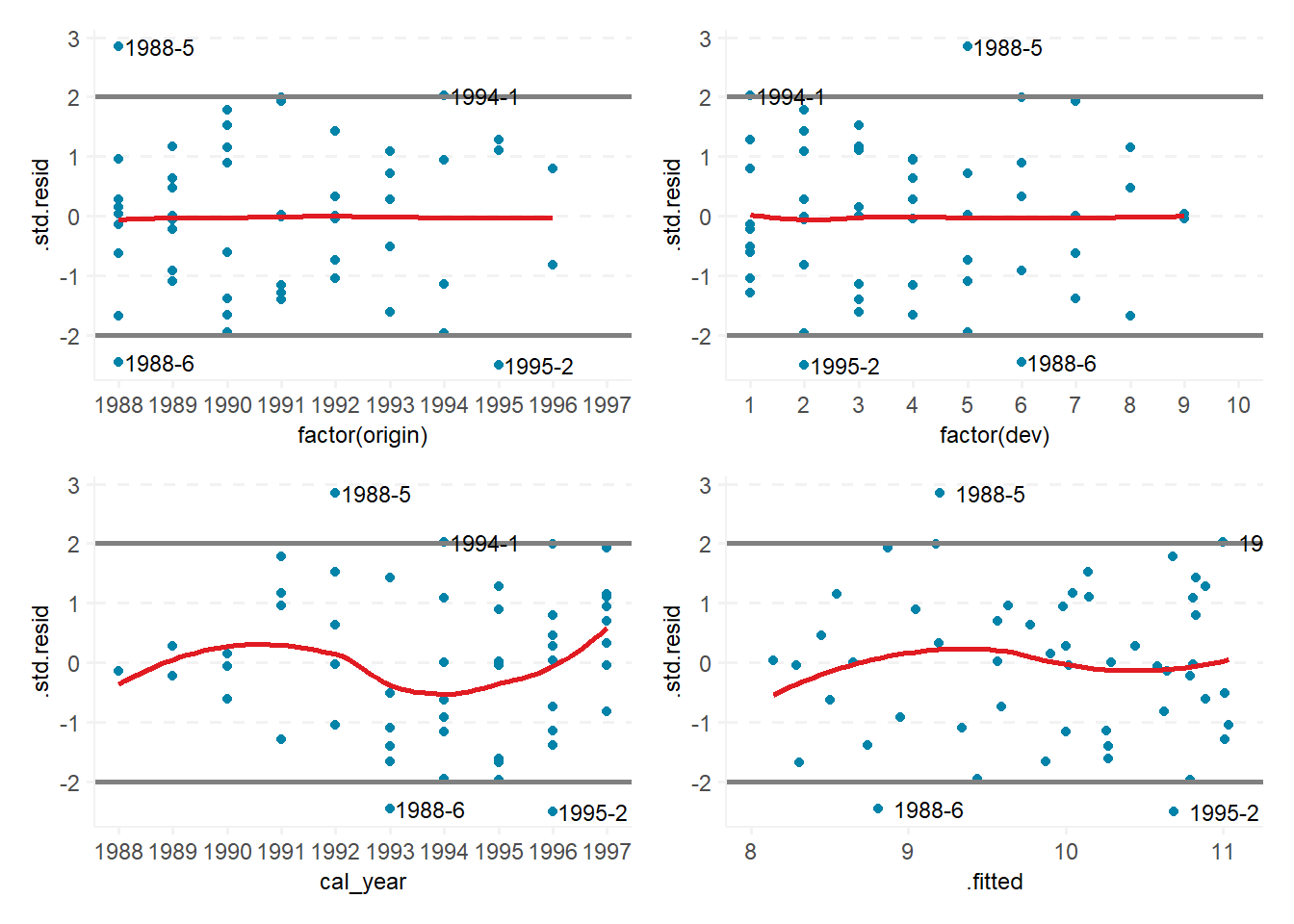

These plots show the standardized residuals versus accident (origin) year, development period, calendar year, and fitted values. All of the plots look reasonable with the residuals randomly centered around zero and only a few outliers in each.

Bayesian chain ladder using `rstanarm`

Now we can take the same GLM formulation, but use Bayesian methods for the estimation. The rstanarm package makes it very straightforward to do this.

First we convert our triangle object to “long” form.

long_paid_tri <- cum2incr(paid_triangle) %>%
  as.data.frame(paid_triangle) %>% 
  filter(!is.na(value))
head(long_paid_tri)
#>   acc_yr dev_lag value
#> 1   1988       1 41821
#> 2   1989       1 48167
#> 3   1990       1 52058
#> 4   1991       1 57251
#> 5   1992       1 59213
#> 6   1993       1 59475

Then we can call the stan_glm function to fit our model.

nb_theta <- est_chainladder_nb$model$theta

est_cl_bayesian_nb <- stan_glm(value ~ factor(acc_yr) + factor(dev_lag),
                            family = neg_binomial_2(link = "log"), 
                            prior_aux = normal(0, nb_theta * 2),
                            data = long_paid_tri)

broom.mixed::tidy(est_cl_bayesian_nb, intervals = TRUE, prob = 0.95) %>% 
  mutate_at(2:3, popformatting::number_format, digits = 3) %>% 
  flextable::regulartable() %>% 
  popformatting::ft_theme() %>% 
  flextable::align(j=1, align="left", part = "all") %>% 
  add_title_header("Bayesian chain ladder parameter summary", 
                   font_size = 18) %>% 
  flextable::fontsize(size = 16, part = "all")

Bayesian chain ladder parameter summary
term	estimate	std.error
(Intercept)	10.648	0.034
factor(acc_yr)1989	0.146	0.032
factor(acc_yr)1990	0.242	0.034
factor(acc_yr)1991	0.370	0.036
factor(acc_yr)1992	0.392	0.037
factor(acc_yr)1993	0.370	0.040
factor(acc_yr)1994	0.356	0.043
factor(acc_yr)1995	0.247	0.048
factor(acc_yr)1996	0.189	0.057
factor(acc_yr)1997	0.045	0.076
factor(dev_lag)2	-0.206	0.031
factor(dev_lag)3	-0.745	0.032
factor(dev_lag)4	-1.016	0.035
factor(dev_lag)5	-1.450	0.038
factor(dev_lag)6	-1.843	0.039
factor(dev_lag)7	-2.147	0.044
factor(dev_lag)8	-2.344	0.046
factor(dev_lag)9	-2.507	0.054
factor(dev_lag)10	-2.654	0.077

We can compare the parameter estimates from our two methods and see that they are in close agreement.

broom.mixed::tidy(est_cl_bayesian_nb, intervals = FALSE) %>% 
  bind_cols(broom::tidy(est_chainladder_nb$model) %>% select(-term, "Standard"=estimate)) %>% 
  select(term, Bayesian = estimate, Standard) %>% 
  mutate(`% error` = Bayesian / Standard - 1) %>% 
  mutate_at(2:3, number_format, digits = 3) %>% 
  mutate_at(4, pct_format) %>% 
  flextable::regulartable() %>% 
  popformatting::ft_theme() %>% 
  flextable::align(j=1, align="left", part = "all") %>% 
  add_title_header("Parameter estimate comparison", font_size = 18) %>% 
  flextable::fontsize(size = 16, part = "all")

Parameter estimate comparison
term	Bayesian	Standard	% error
(Intercept)	10.648	10.648	-0.00%
factor(acc_yr)1989	0.146	0.145	0.82%
factor(acc_yr)1990	0.242	0.241	0.37%
factor(acc_yr)1991	0.370	0.369	0.41%
factor(acc_yr)1992	0.392	0.391	0.28%
factor(acc_yr)1993	0.370	0.369	0.27%
factor(acc_yr)1994	0.356	0.354	0.44%
factor(acc_yr)1995	0.247	0.245	0.88%
factor(acc_yr)1996	0.189	0.186	1.66%
factor(acc_yr)1997	0.045	0.043	5.24%
factor(dev_lag)2	-0.206	-0.206	0.06%
factor(dev_lag)3	-0.745	-0.745	0.06%
factor(dev_lag)4	-1.016	-1.016	0.07%
factor(dev_lag)5	-1.450	-1.450	0.04%
factor(dev_lag)6	-1.843	-1.843	-0.03%
factor(dev_lag)7	-2.147	-2.148	-0.07%
factor(dev_lag)8	-2.344	-2.346	-0.08%
factor(dev_lag)9	-2.507	-2.508	-0.05%
factor(dev_lag)10	-2.654	-2.656	-0.06%

We can also confirm that the reserve estimates produced by both methods are the same.

future_tri <- cum2incr(paid_triangle) %>%
  as.data.frame(paid_triangle) %>% 
  filter(is.na(value)) %>%
  mutate(acc_yr = factor(acc_yr), dev_lag = factor(dev_lag)) %>% 
  select(-value)

post_predict_draws <- future_tri %>% 
  tidybayes::add_predicted_draws(est_cl_bayesian_nb) %>%
  mutate_at(7, as.double)

bayesian_cl_summary <- post_predict_draws %>%
  group_by(acc_yr, .draw) %>% 
  summarise(.prediction = sum(.prediction)) %>% 
  summarise(mean_est = mean(.prediction), sd_est = sd(.prediction), 
            cv = sd(.prediction) / mean(.prediction))

sim_total <- post_predict_draws %>%
  group_by(.draw) %>% 
  summarise(.prediction = sum(.prediction))

bayesian_cl_summary <- bayesian_cl_summary %>%
  bind_rows(tibble(acc_yr = "total", 
                   mean_est = mean(sim_total$.prediction),
                   sd_est = sd(sim_total$.prediction),
                   cv = sd(sim_total$.prediction)/mean(sim_total$.prediction))) %>% 
  mutate(Latest = est_chainladder_nb$summary$Latest, IBNR = mean_est, 
         `S.E.` = sd_est, CV = cv, 
         Ultimate = est_chainladder_nb$summary$Latest + mean_est,
         `Dev.To.Date` = Latest / Ultimate)

bayesian_cl_summary %>% 
  select(`Acc Yr` = acc_yr, Latest, `Dev.To.Date`, Ultimate, IBNR, `S.E.`, CV) %>% 
  mutate_at(c(2,4:6), number_format) %>% 
  flextable::regulartable() %>% 
  popformatting::ft_theme(add_w = 0.0, add_h = 0.00, add_h_header = 0.00) %>%
  flextable::bg(i = nrow(est_chainladder_nb$summary), bg = "#F2F2F2", part = "body") %>% 
  popformatting::add_title_header("Bayesian chain ladder reserve estimate", font_size = 18) %>% 
  flextable::fontsize(size = 16, part = "all")

Bayesian chain ladder reserve estimate
Acc Yr	Latest	Dev.To.Date	Ultimate	IBNR	S.E.	CV
1989	162,903	0.9793075	166,345	3,442	352	0.10232483
1990	176,346	0.9556824	184,524	8,178	591	0.07232153
1991	187,266	0.9252061	202,405	15,139	896	0.05916681
1992	189,506	0.8927995	212,260	22,754	1,207	0.05303895
1993	175,475	0.8460864	207,396	31,921	1,630	0.05107670
1994	159,972	0.7780818	205,598	45,626	2,310	0.05062487
1995	122,811	0.6700935	183,274	60,463	3,271	0.05410145
1996	92,242	0.5319070	173,418	81,176	5,144	0.06337166
1997	43,962	0.2923913	150,353	106,391	8,431	0.07924123
total	1,310,483	0.7774703	1,685,573	375,090	12,163	0.03242720

The 375,090 estimate from the Bayesian method is only 0.44% different than the traditional estimate. Similarly, the total CV of 3.24% is close to the traditional estimate of 3.11%.

Bayesian posterior predictive checks

Using a Bayesian framework allows us to more fully interrogate our model and the assumptions underlying it. We can look at the distribution of parameters and predictions, making valid probabilistic statements about our results.

pp_check(est_cl_bayesian_nb, "ecdf_overlay") + 
  pp_check(est_cl_bayesian_nb, "dens_overlay") +
  pp_check(est_cl_bayesian_nb, "boxplot") +
  plot_layout(ncol = 2)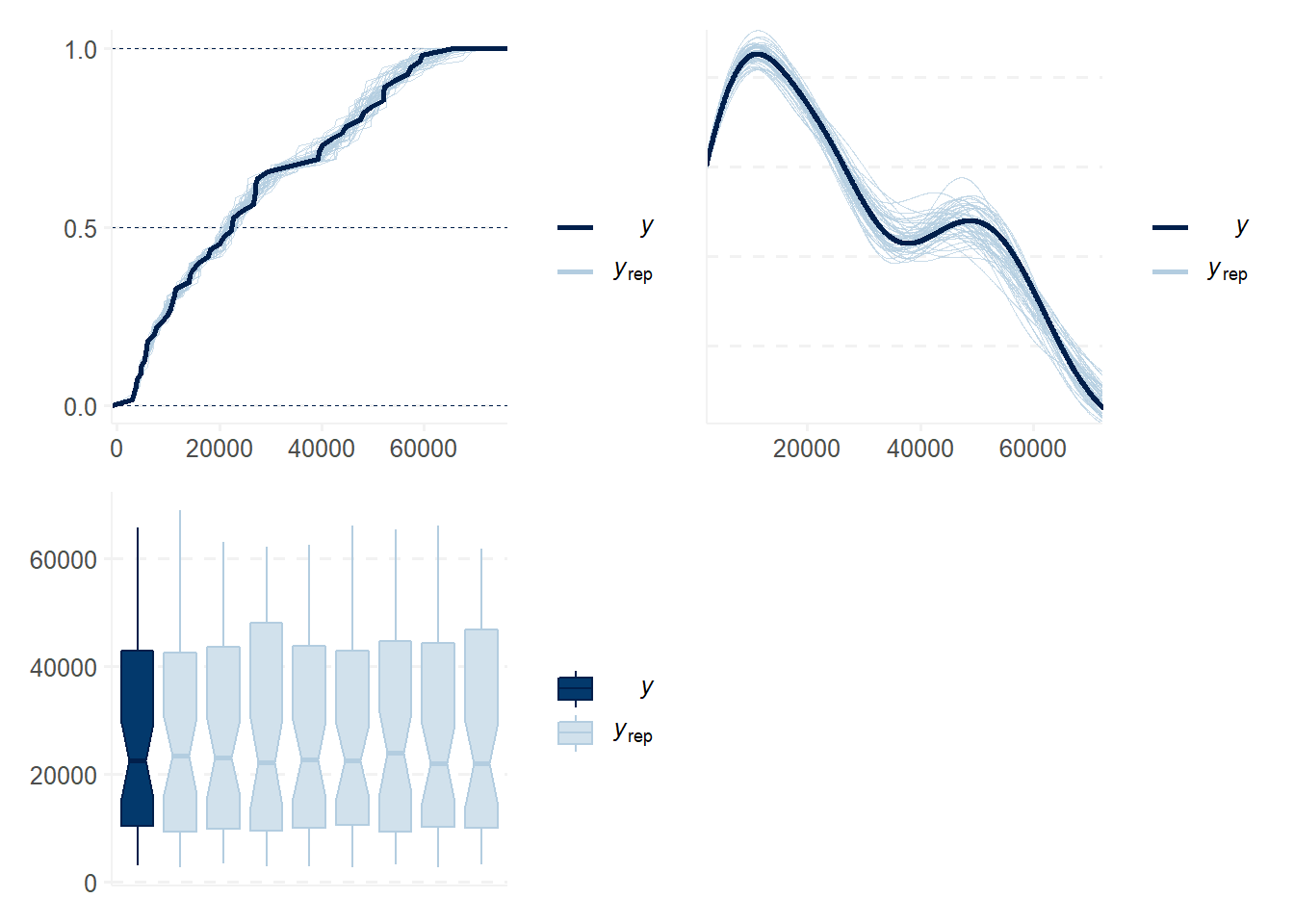

Below is a histogram of the total estimated reserves.

sim_total %>% 
  ggplot(aes(x = .prediction)) +
  geom_histogram() +
  scale_x_continuous(labels = number_format) +
  ggtitle("Distribution of total reserve estimate")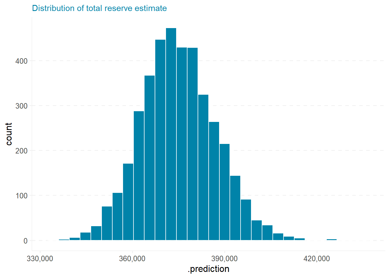

Further enhancements

Now that we have successfully replicated the standard chain ladder method using Bayesian methods, we can move forward taking advantage of the flexibility that the Bayesian framework provides.

For example, we can:

Add informative prior distributions on the parameters
Back-test reserve estimates to determine accuracy in forecasting reserves
Test other distribution families (e.g. Gamma, Skew Normal, etc.)
Add additional variables, such as a calendar year effect